Automatic Obsidian Graph View

During my PhD so far I have been typing notes… A lot of notes. One of the tools I use to make this task more efficient/enjoyable is Obsidian (I actually edit the markdown in Neovim btw). Obsidian is basically a dedicated note taking app that has some very cool features.

One of my favorite features of Obsidian is the ability to link notes. For example, if I’m writing notes on carrots, I can link them to a general note about vegetables. Similarly, a note on how to cook carrot cake can link back to the carrot note.

Obsidian even provides a very pretty view of these notes that they call the Graph View. This view displays notes as interconnected nodes, where each node represents a note file and each link represents the links you specify within the notes.

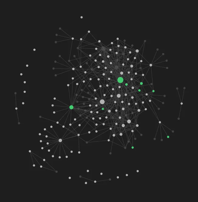
This feature is incredible except for the fact that it relies on one very important factor… That I am actually going to remember to make the link.

So today we are going to explore a little side project that I developped to try and automatically link note files that appear to have similar concepts. This is all done without AI using plain and simple maths and a little too much caffeine.

Inspiration

This coding project was inspired from a live stream I was watching where the streamer, Tsoding, was implementing a research paper called Less is More: Parameter-Free Text Classification with Gzip. This paper aims to use Gzip (which is basically a tool to zip/compress files) to classify a news article as being of a certain category. For example classifying that an article is about science, politics or geography etc.

The stream I was watching by Tsoding can be found here: Zip works Better than AI, and Tsoding’s code can be found here on GitHub. I highly recommend checking out Tsoding’s work, he creates lots of cool projects, generally written in C, however he hates all languages equally which I can respect.

How Does It Work?

First Compressions

Compression is the idea of taking some information, which in our case is a file, and transform that information in such a way that it takes up less physical space in memory.

For example if we have the following string of characters.

aaaabbbccd

This takes up 10 characters. However we could instead transform the string of characters maybe like this.

4a3b2c1d

Where the new string represents the same thing but instead of writing for example four a’s as aaaa we simply say 4a. This is called run length encoding and is one simple example of a compression algorithm.

The run length encoded string only takes up 8 characters meaning we have saved ourselves 2 characters worth of memory, while still representing the same information.

A program, when we want to “decompress” this run length encoded string, can simply transform something like 4a into aaaa and we will get back our original data.

This is one key component of compression algorithms. If we compress a file then decompress it, can we get back the same information? There are some compression algorithms such as JPEG (yep the same one from images) that are lossy and intentionally don’t give back the exact same information after decompression. This trade off allows for JPEG to very aggressively compress the image.

JPEG actually uses the Fourier Transform under the hood to achieve its compression so if you are interested you can check out my previous blog post

However for compressing files, we generally want a lossless compression algorithm. Files could contain any data, it could even be binary, where even just a single changed character could vastly impact the validity of the file.

Gzip is one example of a data compression program that uses lots of complicated compression algorithms under the hood. Windows has its own compression format called zip. For our purposes any compression algorithm will do, but Gzip is what we are going to use.

Kolmogo-Who?

Okay so we know what compression is now.

The paper that I discussed earlier uses a very important concept called Kolmogorov complexity to justify why the particular algorithm works.

The Kolmogorov complexity of an object such as a file (for a completely not foreshadowing reason) is basically the shortest computer program that can be used to represent that file. So for example our run length encoding example from earlier would have low Kolmogorov complexity. Where as a string of random characters would have a higher Kolmogorov complexity because it would be more difficult to write a short program to describe the string.

The above is my understanding of the concept from someone who only recently even heard the term “Algorithmic Information Theory” so if it’s not perfect… My bad.

If you squint your eyes and tilt your head, we can kind of think of compression as being an approximation of Kolmogorov complexity. Where the more the compression algorithm compresses the file, the closer we get to representing the Kolmogorov complexity perfectly.

Similarity Is A Distance?

Using Kolmogorov complexity, a bunch of smart people have come up with a method to compute the distance between two pieces of information. This distance can be interpreted as a similarity. Where the closer the two pieces of information are, the more similar they are and the further apart the more disimilar they are.

There is one small problem with this though. Kolmogorov complexity, can’t actually be computed. However as the paper describes, we can instead compute an approximation of information distance using Gzip as our approximation for Kolmogorov complexity and normalizing.

This is coined the Normalized Compressed Distance (NCD). This is calculated as follows:

\footnotesize NCD(x, y) = \frac{C(xy) - \min(C(x), C(y))}{\max(C(x), C(y))}

I can’t stress this enough. I did not come up with this. This was in the paper I have linked numerous times and all credit goes to authors.

Although it looks intimidating, this algorithm is actually very simple. If we let the operation of “gzipping” something and measuring the length of the result to be given by $C(x)$ where $x$ is the something. Then the min and max operations are used to simply normalize the result around 0-1 (can actually be larger than 1 in reality).

The main distance part of the equation comes from $C(xy)$ . What this part is saying is that if we want to tell the distance between file $x$ and file $y$ , we can glue file $y$ onto the end of file $x$ and then try and compress it. If the files are similar then it should compress a fair bit. Where as if they are dissimilar, then it should’nt compress as much.

For example lets take two files $x$ and $y$ . The contents of $x$ and $y$ are:

x = aaaa

y = aaaa

These files are perfectly similar, so if we compress $xy$ using our run length encoding for a simple example we would get the following:

C(x y) = C(aaaaaaaa)

Which compresses as follows:

RLE(aaaaaaaa) = 8a

Which has a final length of 2. This means that:

C(x y) = C(aaaaaaaa) = 2

Similarly:

C(x) = \text{length}(4a) = 2

C(y) = \text{length}(4a) = 2

So our overall formula becomes:

NCD(x, y) = \frac{2 - \min(2, 2)}{\max(2, 2)} = 0

So x and y have a distance of 0, or they are basically exactly the same.

For another example lets look at the files $x$ and $y$ being given by.

x = aaaa

y = aabb

Which yields

\begin{split} C(xy) & = C(aaaaaabb) \\ & = \text{length}(6a2b) = 4 \end{split}

C(x) = \text{length}(4a) = 2

C(y) = \text{length}(2a2b) = 4

Giving our final distance calculation as

NCD(x, y) = \frac{4 - \min(2, 4)}{\max(2, 4)} = 0.5

Which basically says that they aren’t exactly similar but partly similar.

Piecing It Together

So now that we have a method of quantitatively measuring the similarity between two files, we can finally get on to my idea. I basically wanted to try and recreate Obsidian’s graph view by automatically creating links between the top $n$ files that are most similar to whatever file we are looking at.

I decided to write this project in Rust (btw) and used Axum to serve a web page that displays the graph view using p5.js. I named the project content mapp-rs.

So the main steps were as follows:

Recursively search through all of the files in the current directory (respecting .gitignores).
Gather up all of the paths for the files.
For every combination of file paths compute the NCD.
Remember the $n$ closest/most similar files to whatever file we are currently on. This means they have the smallest NCD.
Turn that into JSON so our front end can make a GET request for it (yes I used polling… Not ideal but good enough)
Draw all of the file connections

The actual node drawing and physics around how the files move in the browser was adapted heavily from a lot of the concepts found in The Nature of Code by Daniel Shiffman who is absolutely amazing if you are interested in anything creative coding.

Oh The Details

The code was implemented after performing some basic optimizations. However unfortunately it was still a little slow for my liking.

In order to improve the processing time I implemented a caching strategy, where instead of computing the Gzip for every single file every time, we instead remember how long a compressed file was. If that comes up again in future computations we can then reuse the value.

While I was already implementing a cache I also cached the date that the file was last modified and decided to save the cache to a file. This allowed me to only rerun the algorithm on files that had actually changed recently or on files that had recently been added. The web server then polls asking for any updated files and redraws them to the screen if any have changed.

Then as my last ditch effort I decided to simply throw more compute at it, I was done trying to come up with clever optimization so now was the time to just brute force it. I sprinkled some parallel computing in there using the amazing Rayon library and just like that I was mostly happy with the performance.

Results

The final product ended up looking like this

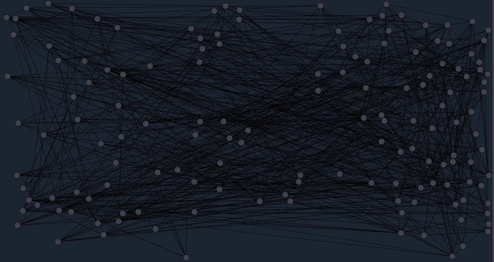
This obviously isn’t quite as pretty as the Obsidian version but I like it.

It seems to work fairly well too! For example:

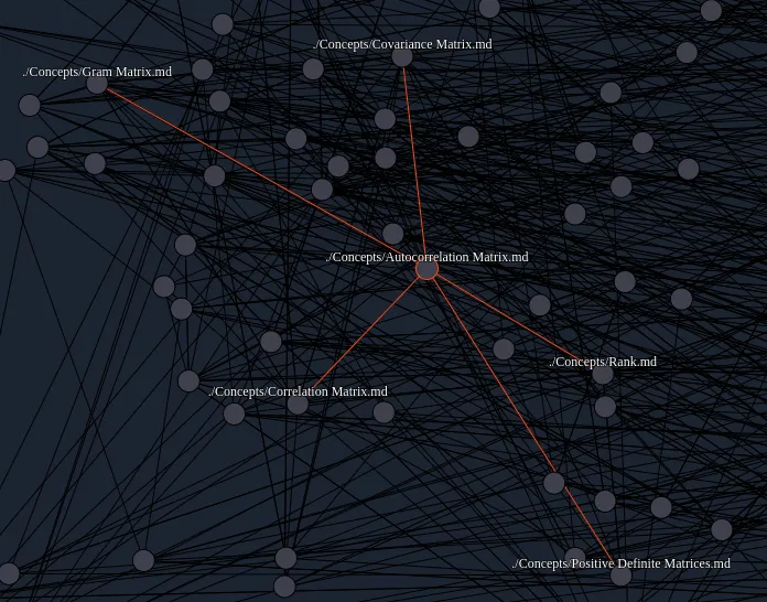
Content Mapp rs automatically detecting similarity

As you can see it correctly identifies that Correlation Matrix, Autocorrelation Matrix, Rank, Covariance Matrix, Gram Matrix and Positive Definite Matrix are all related in some way. Even though I am fairly certain the similarity is mainly based around the use of the word matrix.

Improvements

Because this algorithm is purely based on compression, there is no semantic analysis. This basically means that all NCD’s are computed based purely on how similar the words in one file are to the words in another file. This isn’t how a human would measure similarity though. A human would look at the content of the words, what the words actually mean, and decide how similar the two files are based on that. For example this algorithm could potentially see two files where one describes lead poisoning, and another that describes dog leads as being similar. Purely because they both contain the word lead a lot. Even though as a human we know that lead and lead are two different words (english is fun).

With that being said though, I am very happy with this project and it was a lot of fun for a short project. I hope you all have enjoyed reading about it!

The code for this project can be found on GitHub at Content Mapp-rs. If you have any questions please feel free to open an issue on GitHub.